
DataScience: Study on K-Means and K-Medoids
Introduction:
This report is providing the details analysis of two of the clustering solutions, namely K-means and K-Medoids. Here we are using the 1984 US Congress voting dataset available in mlbench package in R for understanding on how these two clustering solutions work. US Congress voting dataset has 435 observations and 17 different variables. First variable in this dataset contains the class information which provides the details about to which class each of the observation belongs to or voted. So, there are totally 2 different classes/parties to which each observation/person has chosen one among two available parties or classes. There are total of 435 observations and there is some pattern which is followed by remaining 16 variables in choosing the class/party to which each observation has voted. Of the available 435 observations we had 392 observations with missing values/NA either in one or more variables. So, I’m starting my analysis report by performing data preprocessing and then perform clustering on the processed data using various methods available for both clustering and perform comparison study between clustering solutions using available performance measurements and use silhouette values and plots to investigate the cluster stability.
Description:
Data Preprocessing:
Since the available data is not in the best form to perform clustering directly on the data so we need to perform data preprocessing to decide on what we are going to do with missing values in the dataset. We have 3 options here either to ignore the observations with missing values(this is the bad idea as we are going to lose majority of observation as many as 392 out of 435 observations) or substitute “no” to all missing values taking into consideration that people didn’t vote which means they would have voted “no” even if they voted(I’m not considering this point as people might be busy in personal work or other personal related stuff, since we always use the analyzed report for future predictions so we cannot consider people who haven’t voted this time will not vote next time also) and last option we have is imputing the missing values using some of the available algorithms(I’m going with imputing the missing values). After observing the data, I have decided to impute the missing values using “mice” function with random forest method to find best replacement for missing values. We are going with random forest to predict the missing values than Logistic Regression because Random forest is a versatile algorithm (it can do regression also) and can be expected to outperform logistic regression in medium or small dataset. And we are converting the data into binary data(1/0 ‘s).
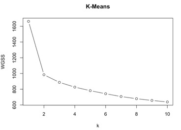
K- Means: Let us start our cluster analysis with K-means. In K-means clustering we select the number of clustering based on the Total Within Group Sum of Squares (WGSS) value. Here I’m calculating WGSS for k = 1 to 10 and after running the algorithm and plotting k vs WGSS I decide to take k = 2 (fig 2). We see from the plot that there is not much variation in selecting k = 2 or k = 3 to 10. Even calculating the Percent of variation, we see that k = 2 has percent of variation which is more when compared to others. After running k-means with different algorithms available such as “Hartigan-Wong”, “Lloyd”, “Forgy” and “MacQueen” we see that “Hartigan-Wong” produced least Total Within Group Sum of Squares for k = 2. So, for K = 2 we have Total Within Group Sum of Square value equals 983.7644 and size of each cluster is 200 and 300 respectively. Misclassification rate suggest that 53 observations have been misclassified, that is ~12% of observation where misclassified. Mean of cluster is 1.46.
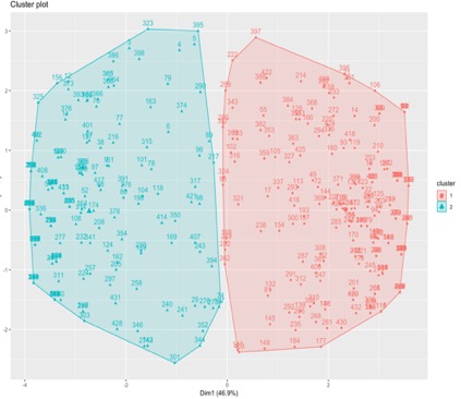
K-Medoids: K-means can be influenced by outliers, however K-Medoids are not influenced by outliers as the use general distance rather than squared distance (used in K-means). Here we won’t decide the number of clusters based on Total Within group sum of square instead we use SWAP to decide the number of clusters. Like we did for K-means we are testing for k = 1 to 10 on different distance methods such as Hamming, Jaccard and Dice. All the three distance methods show that k = 2 is the best option to choose than other k-values. All the swap vs k doesn’t change much for different distance methods. Now let us explore 3 different distance methods separately. Fig.1 shows the k vs SWAP plot and distance used here was Jaccard.
Hamming Distance: Here we calculated the different SWAP values for k = 1 to 10 and we see that k = 2 is the best option to choose as there is not much change in the swap values for k = 2 to 3 than k = 1 to 2. Mean of cluster is 1.528736 and size of cluster shows that there are 205 and 230 observations are classified into cluster 1 and 2 respectively. Maximum and average dissimilarity of cluster 1 are 1.06066 and 0.5849608 respectively and for cluster 2 are 1.0 and 0.6072269. Average diameter of cluster 1 and 2 are 1.274755 and medoid for cluster 1 is 375th observation and 338th observation for cluster 2.
Jaccard Distance: Jaccard method is the default for distance, even here also we choose k = 2. Mean of cluster is 1.51and size of cluster are 210 and 225 observations are classified in to cluster 1 and 2 respectively. Maximum and average dissimilarity of cluster are 0.83 and 0.51 respectively and for cluster 2 are 0.9 and 0.54. Average diameter of cluster 1 and 2 are 0.963 and 0.96, medoid for cluster 1 and 2 are 296th and 10th observation respectively.
Dice Distance: Even Dice distance shows that k = 2 is the best option. Mean for the cluster is 1.51 and size of cluster 210 and 225 observations are classified to cluster 1 and 2 respectively. Maximum and average dissimilarity of cluster are 0.73 and 0.40 respectively and for cluster 2 are 0.83 and 0.42. Average diameter of cluster 1 and 2 are 0.93 and 0.92 respectively, medoid for cluster 1 and 2 are 296th and 10th observation respectively.
From the above 3 different distance methods we see that Dice method has less cluster diameter compared to other 2, similarly all the other values such average and max dissimilarity of cluster are less compared to others. Clusters with less diameter are always better than those cluster with high diameter since cluster with less diameter are tightly packed and all observation have less dissimilarity when compared to those observations in those which has high diameter. From the above output we also see that 2 distance methods such as Jaccard and Dice distance methods had same centroids/medoids and Hamming Distance method had different medoids. When we tabulate clusters of Jaccard and Dice we see that both predicted 210 and 225 observations belongs to cluster 1 and 2 respectively without any misclassification between them. Jaccard and Hamming cluster tabulation shows that both predicted 203 and 223 observations belong to cluster 1 and 2 respectively however, k-medoid using Jaccard predicted 7 observations belong to cluster 1 and 2 observations belong to cluster 2 but these where predicted in opposite cluster by k-medoids using Hamming distance. Tabulation of k-medoids cluster using Hamming and Dice is same as above Hamming and Jaccard distance because Jaccard and Dice predicted same observations in each cluster. Average silhouette width of total data set for k-medoids with Jaccard, Hamming and Dice distance is 0.3606868, 0.3587612, 0.282026. Having higher silhouette (~1) means data was well cluster, but when we compare between above three values k-medoids, Jaccard distance has better clustered data than others. Fig 4 shows the cluster obtained from K-Medoids with Jaccard Distance.
Silhouette:
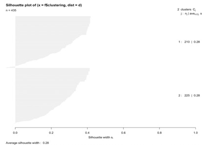
Silhouette tell us how well the clustering was done, Silhouette close to 1 indicates that the data was clustered well else if Silhouette value close to -1 indicates that data/observation would be more appropriate to assign to another cluster. Silhouette value equal to 0 indicates data/observation lies on the boundary of 2 clusters.
| Jaccard Distance | Cluster 1 | Cluster 2 | Cluster 3 | Cluster 4 | Average |
|---|---|---|---|---|---|
| K = 2 | 0.28 | 0.28 | 0.28 | ||
| K = 3 | 0.28 | 0.02 | 0.25 | 0.2 | |
| K = 4 | 0.05 | 0.01 | 0.25 | 0.18 | 0.12 |
Here we see that when K = 4 there are more negative silhouette value for observations in cluster 2, similarly when K = 3 we see that there are more negative silhouette values for observations in cluster 2. Even when K = 2 we have few negative values for cluster 2(fig 3), but since the average silhouette value for K = 2 is more than others so we can say that compared to K = 3 or 4 we can say that in K = 2 clustering was well performed. Similarly, all the below tables show that average silhouette values are more for K = 2 compared to other values of K.
| Hamming Distance | Cluster 1 | Cluster 2 | Cluster 3 | Cluster 4 | Average |
|---|---|---|---|---|---|
| K = 2 | 0.37 | 0.35 | 0.36 | ||
| K = 3 | 0.37 | 0.23 | 0.03 | 0.24 | |
| K = 4 | 0.08 | 0.22 | 0.04 | 0.14 | 0.13 |
| Dice Distance | Cluster 1 | Cluster 2 | Cluster 3 | Cluster 4 | Average |
|---|---|---|---|---|---|
| K = 2 | 0.36 | 0.36 | 0.36 | ||
| K = 3 | 0.35 | 0.02 | 0.29 | 0.24 | |
| K = 4 | 0.05 | 0.009 | 0.29 | 0.21 | 0.13 |
| Euclidean(K-Means) | Cluster 1 | Cluster 2 | Cluster 3 | Cluster 4 | Average |
|---|---|---|---|---|---|
| K = 2 | 0.54 | 0.57 | 0.55 | ||
| K = 3 | 0.51 | -0.03 | 0.57 | 0.41 | |
| K = 4 | 0.53 | 0.40 | 0.11 | 0.01 | 0.32 |
Here we see that K-Means with 2 cluster has best average silhouette value compared others which means that K-Means has well clustered data compared to others.
Adjusted Rand Index:
Adjusted Rand Index is a number between 0 and 1 and is used to compare agreement between two clustering solutions. Below table shows that adjusted Rand Index between pair of clustering solutions for k = 2. Here K-medoids are represented as KD and K-means as KM.
| KD(Jaccard) | KD(Hamming) | KD(Dice) | KM(Euclidean) | |
|---|---|---|---|---|
| KD(Jaccard) | 1 | |||
| KD(Hamming) | 0.91 | 1 | ||
| KD(Dice) | 1 | 0.91 | 1 | |
| KM(Euclidean) | 0.91 | 0.90 | 0.91 | 1 |
Above table is symmetric matrix, here we see that most of the pair clusters have strong agreement between them and we can see that K-Medoids with Dice and Jaccard distance have strongest agreement between them (we have seen in the medoids sections that both of them divided the same observations into 2 clusters).
Conclusion:
In the above analysis we have discussed about various concepts, we have discussed about K-Means and K-Medoids and in K-medoids we explored various available distance methods. Misclassification rate by K-Means is 12.3%, K-Medoids with Jaccard distance is 12.8%, K-Medoids with Hamming distance is 14.4% and K-Medoids with Dice distance is 12.8%. After various comparison study on number of clusters to choose all the methods influenced us to consider 2 clusters would be better than going with higher number. And we have seen that K-Medoids with Dice had produced clusters with less diameter (observations are tightly packed). Silhouette plot shows that K-Means has highest average silhouette value than others, which tell us that clustering was best in K-Means than other methods. We have also seen that adjusted Rand Index for different distance methods and we can say that K-medoids with Dice and Jaccard produced same results, and we saw that all of the methods have strong agreement between them from adjusted Rand Index. From all these computations I would like conclude stating we would use K-Means to cluster the US Congress Voting dataset as we have less misclassification rate and highest average silhouette value compared to others.
Plots:
Plot-1

Plot-2
Plot-3
Plot-4